
Dear All,
Every semester we crack our heads trying to grade students’ exam scripts, totalling up the marks and then converting the marks into grades (A, A-, B+ etc). Later we have to convert the grades into grade points and then calculate Cumulative Grade Point Average (CGPA) for each student. Usually we do all that manually, ending up with many mistakes which causes unnecessary embarassment to us and the department. So I would like to introduce the following Excel command which we can use.
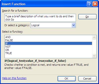
IF(logical_test,value_if_true,value_if_false)
or
IF(logical_test;value_if_true;value_if_false)
Whether to use “;” or “,” as the separating syntax depends on the version of Excel being used.
We use quotation marks (” “) to bracket the outcome values only if the outcome is categorical, for example “PASS”.
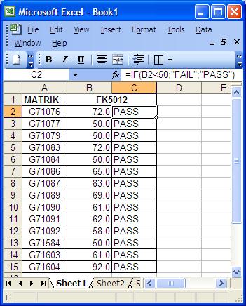
=IF(B2<50;”FAIL”;”PASS”)
If the outcome values is continuous data, then we don’t have to use quotation marks. For example;
=IF(B2<50;0;1)
For more information about the command, just highlight the command and click on “Help on this function”. You will get the following explaination;
| Info From Excel Help File
IF Returns one value if a condition you specify evaluates to TRUE and another value if it evaluates to FALSE. Syntax IF(logical_test,value_if_true,value_if_false) Logical_test is any value or expression that can be evaluated to TRUE or FALSE. For example, A10=100 is a logical expression; if the value in cell A10 is equal to 100, the expression evaluates to TRUE. Otherwise, the expression evaluates to FALSE. This argument can use any comparison calculation operator. Value_if_true is the value that is returned if logical_test is TRUE. For example, if this argument is the text string “Within budget” and the logical_test argument evaluates to TRUE, then the IF function displays the text “Within budget”. If logical_test is TRUE and value_if_true is blank, this argument returns 0 (zero). To display the word TRUE, use the logical value TRUE for this argument. Value_if_true can be another formula. Value_if_false is the value that is returned if logical_test is FALSE. For example, if this argument is the text string “Over budget” and the logical_test argument evaluates to FALSE, then the IF function displays the text “Over budget”. If logical_test is FALSE and value_if_false is omitted, (that is, after value_if_true, there is no comma), then the logical value FALSE is returned. If logical_test is FALSE and value_if_false is blank (that is, after value_if_true, there is a comma followed by the closing parenthesis), then the value 0 (zero) is returned. Value_if_false can be another formula. Remarks
|
Utilising the above command, you can come up with a simple command which will discriminate whether the students have passed or failed the exam by using the following example, (using B as the column where the marks are entered and entering the formula in box C2);
=IF(B2<50;”FAIL”;”PASS”)
Since we have to discriminate into various grades, instead of just PASS & FAIL, we have to create a more complicated version of the command.
To illustrate a more complicated command, I shall use the department’s Postgraduate Diploma in Occupational Health (DSKP) programme as an example.
Identifying the Criterion
| Criteria set by the DSKP programme |
Cutoff point (confirm with supervisor) |
GPA |
| A = 80 and above A- = 75 – 79 B+ = 70 – 74 B = 65 – 69 B- = 60 – 64 C+ = 55 – 59 C = 50 – 54 E = Less than 50 |
A > 79.9999 A- = 75 – 79.9999 B+ = 70 – 74.9999 B = 65 – 69.9999 B- = 60 – 64.9999 C+ = 55 – 59.9999 C = 50 – 54.9999 E <50 |
4.00 3.67 3.33 3.00 2.67 2.33 2.00 0.00 |
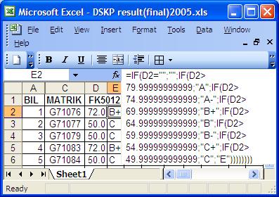
Assuming that the marks were in column D, the grades were in column E and the GPA in column F, based on the above, we should use the following command for grades in box E2;
=IF(D2=””;””;IF(D2>79.9999;”A”;IF(D2>74.9999;”A-“;IF(D2>69.9999;”B+”;IF(D2>64.9999;”B”;IF(D2>59.9999;”B-“;IF(D2>54.9999;”C+”;IF(D2>49.9999;”C”;”E”))))))))
For GPA, we should use the following command in box F2;
=IF(E2=””;””;IF(E2=”A”;4;IF(E2=”A-“;3.67;IF(E2=”B+”;3.33;IF(E2=”B”;3;IF(E2=”B-“;2.67;IF(E2=”C+”;2.33;IF(E2=”C”;2;0))))))))
Please note that I already used the maximum of 7 nested commands to categorise the marks into 8 categories. To complete the job, highlight box E2 and F2 together and drag the commands into the lower boxes.
Looks complicated but since the above example is already available, just “copy & paste” 🙂
Since the Department of Community Health runs many postgraduate programmes besides the undergraduate programme, let us identify the suitable commands for a few of the other programmes such as the undergraduate, Masters of Community Health (SKM) and Masters of Science of Community Health (SSKM).
Undergraduate
| Criteria set for u/grad programme |
Cutoff point (based on my observation) |
| A = 80 and above A- = 75 – 79 B+ = 70 – 74 B = 65 – 69 B- = 60 – 64 C+ = 55 – 59 C = 50 – 54 C- = 47 – 49 D+ = 44 – 46 D = 41- 43 E = 40 or less |
A > 79.4999 A- = 74.5 – 79.4999 B+ = 69.5 – 74.4999 B = 64.5 – 69.4999 B- = 59.5 – 64.4999 C+ = 54.5 – 59.4999 C = 49.5 – 54.4999 C- = 46.5 – 49.4999 D+ = 43.5 – 46.4999 D = 40.5 – 43.4999 E <40.5 |
The weird thing about the undergraduate programme is that, although the marks are entered into the faculty system up to a single decimal point, it will be rounded up (no decimal point) by the software for the grades. To ensure our grades and the faculty grades tally, I came up with the above cutoff points, based on my observation of the final results.
Please note that there are a total of 11 categories of grades. Just for the 8 grades in DSKP, we already utilised the maximum 7 nested commands. For the DSKP programme, I start from the maximum value and then went one way only towards lesser values. So for 11 categories of grades, the nesting of commands becomes much more complex. I intially divide the marks into two groups, then I start nesting the commands two ways for both outcome.
Assuming the marks were in column U and the grades were in column V, please enter the following command in box V2;
=IF(U2>59.4999;IF(U2>79.4999;”A”;IF(U2>74.4999;”A-“;IF(U2>69.4999;”B+”;IF(U2>64.4999;”B”;”B-“))));IF(U2<40.5;IF(U2=””;””;”E”);IF(U2<43.5;”D”;IF(U2<46.5;”D+”;IF(U2<49.5;”C-“;IF(U2<54.5;”C”;”C+”))))))
Since the programme is being run by the Academic Department, we don’t have to worry about CGPA. To complete the job, highlight box V2 and drag the command into the lower boxes.
Postgraduate – Masters of Community Health (SKM)
| Criteria set by the SKM programme |
Cutoff point (confirm with supervisor) |
| A = 80 and above A- = 70 – 79 B = 60 – 69 C = 50 – 59 D < 50 E = absent |
A > 79.9999 A- = 70 – 79.9999 B = 60 – 69.9999 C = 50 – 54.9999 D < 50 E = “” |
Please note that there are a total of 6 categories of grades. So we just need an abbreviated version of the DSKP command. Assuming the marks were in column U and the grades were in column V, please enter the following command in box V2;
=IF(U2>49.9999;IF(U2>79.9999;”A”;IF(U2>69.9999;”A-“;IF(U2>59.9999;”B”;IF(U2=””;”E”;”C”))));”D”)
SKM has no CGPA IIANM. To complete the job, highlight box V2 and drag the command into the lower boxes.
Postgraduate – Masters of Science of Community Health (SSKM)
| Criteria set by the SSKM programme |
Cutoff point (confirm with supervisor) |
GPA |
| A = 80 and above A- = 75 – 79 B+ = 70 – 74 B = 65 – 69 B- = 60 – 64 C+ = 55 – 59 C = 50 – 54 C- = 45 – 49 D = 40 – 44 E = 39 or less |
A > 79.9999 A- = 75 – 79.9999 B+ = 70 – 74.9999 B = 65 – 69.9999 B- = 60 – 64.9999 C+ = 55 – 59.9999 C = 50 – 54.9999 C- = 45 – 49.9999 D = 40 – 44.9999 E < 40 |
4.00 3.67 3.33 3.00 2.67 2.33 2.00 1.67 1.00 0.00 |
Please note that there are a total of 10 categories of grades. So we just need an abbreviated version of the undergraduate command. Assuming the marks were in column U, the grades were in column V and the GPA in column W, please enter the following command in box V2;
=IF(U2>59.9999;IF(U2>79.9999;”A”;IF(U2>74.9999;”A-“;IF(U2>69.9999;”B+”;IF(U2>64.9999;”B”;”B-“))));IF(U2<40;IF(U2=””;””;”E”);IF(U2<45;”D”;IF(U2<50;”C-“;IF(U2<55;”C”;”C+”)))))
For GPA, we should use the following command in box W2;
=IF(V2=”A”;4;IF(V2=”A-“;3.67;IF(V2=”B+”;3.33;IF(V2=”B”;3;IF(V2=”B-“;2.67;IF(V2=”C+”;2.33;IF(V2=”C”;2;IF(V2=”C-“;1.67;0))))))))
Unfortunately this command will give a GPA of 0.00 for missing, D and E. This can’t be avoided since we can do only a maximum of 7 nested command of “IF…THEN”. Therefore we have to manually check and correct the GPA for “D” only.
To overcome this, we can use the following command in box W2;
=IF(U2>59.9999;IF(U2>79.9999;4;IF(U2>74.9999;3.67;IF(U2>69.9999;3.33;IF(U2>64.9999;3;2.67))));IF(U2<40;IF(U2=””;””;0);IF(U2<45;1;IF(U2<50;1.67;IF(U2<55;2;2.33)))))
To complete the job, highlight box V2 and W2 together and drag the commands into the lower boxes.
Calculating the CGPA
IIANM the CGPA is calculated by multiplying the GPA to the course unit, total up and then divided by the total units of the semester. For example;
CGPA = (SUM of unit*GPA)/Total Unit
Using the DSKP programme as an example;
| Module | Unit | Location in Excel Sheet |
| FK5012 | 2 | F |
| FK5112 | 2 | I |
| FK5212 | 2 | L |
| FK5314 | 4 | O |
| FK5022 | 2 | R |
| FK5122 | 2 | U |
| FK5222 | 2 | X |
| FK5322 | 2 | AA |
| FK5422 | 2 | AD |
| FK5032 | 2 | AG |
| FK5132 | 2 | AJ |
| FK5232 | 2 | AM |
| FK5234 | 4 | AP |
| TOTAL | 30 |
=(2*F2+2*I2+2*L2+4*O2+2*R2+2*U2+2*X2+2*AA2+2*AD2+2*AG2+2*AJ2+2*AM2+4*AP2)/30
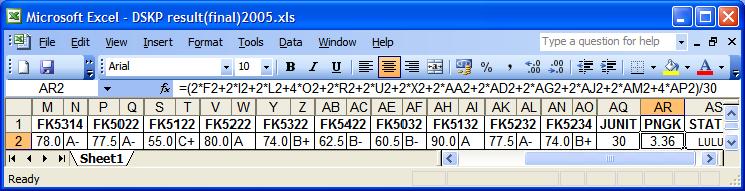
To complete the job, highlight box AR2 and drag the command into the lower boxes.
Conclusion
Life is already too hard. Let’s keep it simple.